In machine learning, it’s common to scale data (especially predictor variables (IVs)) to ensure consistency in model application and interpretation.
Standardisation and normalisation are techniques that scale the data. They do it in slightly different ways, which can significantly impact the performance of the ML algorithms.
80.2 Standardisation
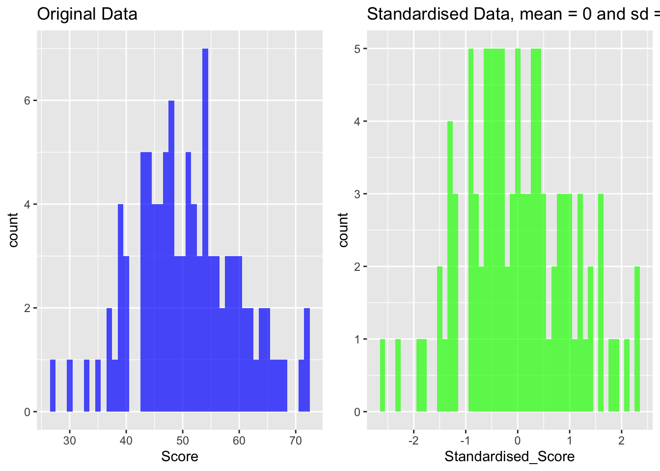
Standardisation involves shifting the distribution of each variable to have a mean of 0 and a standard deviation of 1.
It’s especially useful for algorithms that assume data is normallydistributed, like logistic regression or linear regression.
We can use the scale function in R to standardise our data.
An example for one variable
# Load necessary librarylibrary(ggplot2)# Create sample dataset.seed(123)data <-data.frame(Score =rnorm(100, mean =50, sd =10))# Standardise a vector in the datasetdata$Standardised_Score <-scale(data$Score)# Plot original vs. standardised datap1 <-ggplot(data, aes(x = Score)) +geom_histogram(binwidth =1, fill ="blue", alpha =0.7) +ggtitle("Original Data")p2 <-ggplot(data, aes(x = Standardised_Score)) +geom_histogram(binwidth =0.1, fill ="green", alpha =0.7) +ggtitle("Standardised Data, mean = 0 and sd = 1")gridExtra::grid.arrange(p1, p2, ncol =2)
An example where all predictors are scaled
# Create sample dataframeset.seed(123) data <-data.frame(Variable1 =rnorm(100, mean =20, sd =5),Variable2 =runif(100, min =10, max =50),Variable3 =rnorm(100, mean =0, sd =1),Variable4 =rbinom(100, size =10, prob =0.5),Variable5 =runif(100, min =0, max =100) # This variable will not be scaled)# Scale first four variables by creating another dataframedata_scaled <-as.data.frame(lapply(data[1:4], scale))# Add the unscaled Variable5 back into the scaled dataframedata_scaled$Variable5 <- data$Variable5# Display scaled datahead(data_scaled)
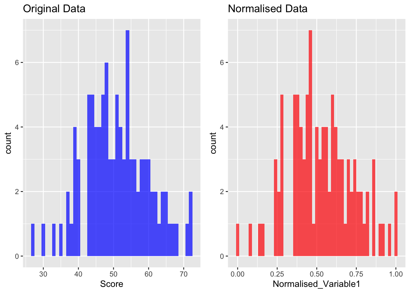
Normalisation adjusts the scale of the data so that the range is between 0 and 1.
This is useful for algorithms that compute distances between data points, like K-Nearest Neighbors (KNN) and K-Means clustering.
We can use ‘min-max scaling’ in R to achieve this.
# using the same dataset created above# normalise data using min-max data$Normalised_Variable1 <- (data$Variable1 -min(data$Variable1)) / (max(data$Variable1) -min(data$Variable1))# plot original vs. normalisedp3 <-ggplot(data, aes(x = Normalised_Variable1)) +geom_histogram(binwidth =0.02, fill ="red", alpha =0.7) +ggtitle("Normalised Data")gridExtra::grid.arrange(p1, p3, ncol =2)
80.4 When to use
The choice between standardisation and normalisation depends on the characteristics of your data and the requirements of the algorithm you’re using.
We typically standardise data when you’re dealing with features that have a Gaussian (bell curve) distribution. Standardisation is important for models that assume that all features are centered around zero and have variance in the same order, such as:
Linear Regression
Logistic Regression
Support Vector Machines
Principal Component Analysis (PCA)
Algorithms that compute distances or assume normality
Normalisation rescales the data into a range of [0, 1] or [-1, 1]. It’s useful when you need to scale the features so they’re in a bounded interval.
Normalisation is often the choice for models that are sensitive to the magnitude of values and where you don’t assume any specific distribution of features, such as:
Neural Networks
k-Nearest Neighbors (k-NN)
k-Means Clustering
Situations where you need to maintain zero entries in sparse data.
In practice, I’d suggest that you try both methods as part of your exploratory data analysis to determine which scaling technique works better for your specific model and dataset.